Target Population and Samples
The target population covered in the SOEP is defined as the residential population living in private households within the current boundaries of the Federal Republic of Germany (FRG). Because of changes in these boundaries (in 1990) and changes in the residential population due to migration, various adaptations have been applied to the initial sampling structure to keep the sample’s representativity. In addition, certain groups have been oversampled to increase the statistical power.
In 1984, the survey started with a sample covering the entire population in then West Germany (FRG), where the five biggest groups of foreigners (the so-called “guestworkers”) were oversampled.
The institutionalized population, in the true sense of the word (hospitals, nursing homes, military installations) is generally not representatively included in new samples. E.g. in 1984 only 57 institutionalized households are included. Later, however, persons from the initial households who have taken up residence temporarily or permanently in institutions of this kind are followed. For a detailed description of the problems in covering this population in the SOEP, see Hanefeld (1987).
The SOEP was expanded to the territory of the German Democratic Republic in June 1990, only six months after the fall of the Berlin Wall. A further addition in 1994/95 was a sample of migrants who came to Germany after 1984, to take the influx of ethnic Germans from former Soviet countries into account. Two samples respresentative of the entire population in Germany were added in 1998 and 2000, to counter effects of panel attrition and to increase the overall sample size. In 2002, a high income sample was added, while in 2006 and 2009, additional refreshment samples were drawn.
To increase the overall sample size SOEP has started adding refreshment samples in 2011. While the first (in 2011) and second (2012) extensions are representative of the whole population, the third (2013) is supposed to explicitly cover migrants. For the fourth extension in 2014, the related study “Families in Germany”, covering mainly families, will be integrated into the SOEP.
The different samples in the SOEP are identified by letters: sample “A” refers to the German sample drawn in 1984, “C” to the East Germans from 1990, and so on. Even though these samples are kept separate, the respondents recieved identical questionnaires for the most part and distinctions by sample are usually not be necessary in an analysis.
However, one of the ideas of SOEP is, that the users have full information available about survey methodological issues and survey design. Which means in this case that you can of course identify the corresponding sample for each observation. In the following section, we present details on each of the samples, which - unless stated otherwise - are multi-stage random samples with regional clusters. The respondent’s households are selected by random-walk routines. For an extensive discussion on sampling (and weighting) see @Kroh2012.
i. The SOEP Samples in Detail
Sample A “Residents in the FRG” covers persons in private households with a household head, who does not belong to one of the main foreigner groups of “guestworkers” (i.e. Turkish, Greek, Yugoslavian, Spanish or Italian households). Because only a few foreigners are in Sample A it is often called the “West German Sample” of the SOEP. In 1984 it covered 4,528 households with a sampling probability of about 0.0002.
Sample B “Foreigners in the FRG” adds persons in private households with a Turkish, Greek, Yugoslavian, Spanish or Italian household head, which in 1984 constituted the main groups of foreigners in the FRG. Compared to Sample A the population of Sample B is oversampled with a sampling probability of about 0.002. The first wave included 1,393 households in Sample B.
Sample C “German Residents in the GDR” consists of persons in private households where the household head was a citizen of the German Democratic Republic (GDR). This meant that approximately 1.7% of the residential population in the GDR in June 1990 was excluded from the sample as foreigners (who were mostly institutionalized). All in all, 2,179 households represent the starting size of this sample with a sampling probability of about 0.0005.
Sample D “Immigrants” started in 1994/95 with two different samples. In 1994, the first sample D1 had 236 households and in 1995, the second sample D2 had 295 households, leading to a total of 531 households (D1 and D2) in 1995. This sample consisted of households in which at least one household member had moved from abroad to West Germany after 1984. The sampling probability is about 0.0002.
Sample E “Refreshment” was added in 1998, selected from the entire population of private households in Germany. The households were chosen independently from the ongoing panel and its subsamples A through D, with the targets of increasing the number of observations of the general population and preserving its representativity. The selection scheme used for sample E essentially resembles the one used in subsample A. The number of households in the first wave of subsample E was \(1,060\), with a sampling probability of about 0.00005. With the data distribution of 2012, parts of subsample E have been extracted into the SOEP Innovation Sample.
Sample F “Refreshment” was selected independently from all other subsamples from the population of private households in 2000. The selection scheme was slightly altered compared to the previous addition in Sample E: while the ’German’ households (all adults greater or equal 16 in the household have German nationality) were selected with a sampling probability of \(0.00028\), the ’non-German’ households (at least one adult does not have German nationality) where oversampled with a probability of 0.0005. Overall, the number of added households in subsample F’s first wave amounts to 6,043.
Sample G “High Income” entered the SOEP in 2002 independently from all other subsamples. The original selection scheme required that the responding households had a monthly income of at least DM 7,500 (EUR 3,835), which - due to the lack of an adequate sampling frame - were identified using a screening procedure. This sample of overall 1,224 households increased the potential for analyses in the high income areas, which previously were difficult to conduct because of low case numbers. The derived sampling probability is about 0.0014. Starting with Wave 2 in 2003, the selection scheme for this subsample was changed such that only households with a net monthly income of at least EUR 4,500 were followed.
Sample H “Refreshment” started in 2006 as a random sample, again independently of all previous subsamples, covering all residential households in Germany. The addition of 1,506 households was drawn with a sampling probability of 0.0001.
Sample I “Incentive sample” started in 2009, where in the first wave, a new incentive scheme was tested to increase participation rates (see also [sec:PanelCare]. The sampling was independent of all other SOEP-samples, adding a total number of 1,531 households to the SOEP. Their sampling probability was 0.00013. This sample remained in the main data distribution for its first two waves (i.e. 2010 and 2011, or waves Z and BA). With the data distribution of 2012, subsample I has been extracted into the SOEP Innovation Sample.
Sample J “Refreshment sample” started in 2011 as a random sample that was drawn independently of all previous subsamples, covering the residential households in Germany. The addition of 3,136 households was drawn with a sampling probability of 0.0002.
Sample K “Refreshment sample” started in 2012 as a random sample, drawn independently of all previous subsamples, covering the residential households in Germany. The addition of 1,526 households was drawn with a sampling probability of 0.0001.
In 2013 a new migration sample was added with around 2,700 households drawn by using register information of the German Federal Employment Agency.
ii. Eligibility and Follow-up
As mentioned, the SOEP’s goal is to be representative of the residential population of Germany. All household members 16 and older are eligible for a personal interview, starting with the youth questionnaire at that age, followed by “regular” person questionnaires thereafter. As years go by, the children of the first wave reach age-eligibility and become panel members. If they move out and form their own families, they and their new families are still part of the survey. “New” persons become part of the SOEP population due to birth or residential mobility. In case a person enters a SOEP household after the initial wave, this person is asked to fill out the regular person questionnaire if age-eligible, or will be asked to participate once old enough. Thus in the absence of panel attrition the SOEP would be a self-sustaining survey.
The concept of how to follow the respondents and sample members over time is important for the representativeness of the study. The basic principle for follow-up in the SOEP is that all persons participating in a wave of any subsample are to be surveyed in the following years as long as they stay within the boundaries of Germany. This rule also extends to respondents who entered a SOEP-household after the first wave due to residential mobility or birth. If there is a “split-off”, i.e. people move out of the household they were last interviewed in, the members of the new household receive a new household identifier. Table 3 conceptualizes how new sample members and households are realized in the SOEP. Figure 2 shows that as a result of the follow-up concept, up to , several thousand “new” households became part of the SOEP population. The weighting scheme takes into account this complete “follow-up” (see @Kroh2012).
Persons or households who could not be interviewed in a given year are termed “temporary drop-outs”. These are followed until there are two consecutive waves of missing interviews for all household members or a final refusal of the complete household. In the case of a cooperation after a temporary drop-out, the respondent is asked to fill out an additional short questionnaire on central information on employment and demographics during the year of absence.
Table 3: Changes to the Sample: Respondents and Households
| Existing Households | New Households | |
|---|---|---|
| Existing Persons | “classic case”: without change of address entire household moves | Move-out |
| New Persons | Birth Move-in | Move-in or birth into move-out household |
Figure 2: Old and New Households in the SOEP 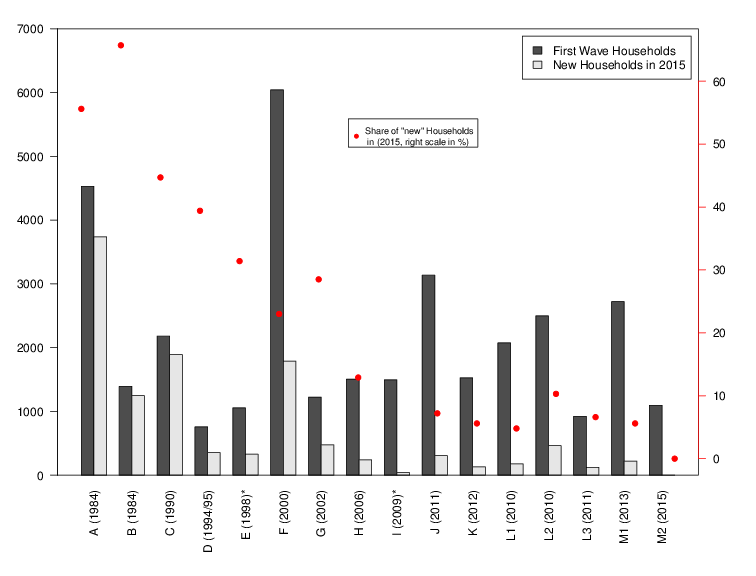 R Code to create figure.
Development of Sample Sizes
Individuals who refuse participation or are not available for an interview are kept in the so-called “gross” sample of the study as long as they continue to live in households with at least one participating person. Once the entire household declines to respond in two consecutive waves of data collection, all individuals from the household are removed from the SOEP. Table 4 shows the starting sample sizes of samples A through J, the years when the samples were first collected, as well as the percentage of those persons who were eligible for an interview but declined participation (“partial unit non-response”, PUNR) in the first wave. Figure 3 illustrates the development of the number of successful person interviews since 1984. The reduction in the population size for all individual samples is mainly the result of person-level drop-outs, refusals, moving abroad, etc. However, due to new persons moving into already existing households, and children reaching the minimum respondent’s age of 16, and thereby increasing the sample size, this negative development is offset somewhat.
Table 4: Starting Sample Size of the SOEP Samples
| Sample | Year | Households (net) | Persons (gross) | Respondents (net) | Partial Unit Non-response (percent) | Children (gross) |
|---|---|---|---|---|---|---|
| A | 1984 | 4,528 | 11,422 | 9,076 | 0.6 | 2,290 |
| B | 1984 | 1,393 | 4,830 | 3,169 | 0.7 | 1,638 |
| C | 1990 | 2,179 | 6,131 | 4,453 | 1.9 | 1,591 |
| D1 | 1994 | 236 | 733 | 471 | 2.9 | 248 |
| D1/D2 | 1995 | 541 | 1,668 | 1,078 | 6.1 | 517 |
| E | 1998 | 1,057 | 2,446 | 1,910 | 3.5 | 466 |
| F | 2000 | 6,043 | 14,510 | 10,880 | 5.5 | 2,991 |
| G | 2002 | 1,224 | 3,538 | 2,671 | 6.1 | 693 |
| H | 2006 | 1,506 | 3,407 | 2,616 | 6.0 | 623 |
| I | 2009 | 1,495 | 3,428 | 2,432 | 13.4 | 620 |
| J | 2011 | 3,136 | 6,873 | 5,161 | 9.9 | 1,147 |
| L1 | 2010 | 2,074 | 7,939 | 3,770 | 6.7 | 3,900 |
| L2 | 2010 | 2,500 | 9,063 | 4,227 | 5.1 | 4,611 |
| L3 | 2011 | 924 | 3,645 | 1,487 | 4.2 | 2,092 |
| K | 2012 | 1,526 | 3,286 | 2,473 | 9.2 | 563 |
| M1 | 2013 | 2,723 | 8,522 | 4,964 | 17.8 | 2,481 |
| M2 | 2015 | 1,096 | 3,048 | 1,711 | 19.3 | 927 |
Figure 3: Cross-Sectional Development of Sample Size (Respondents)

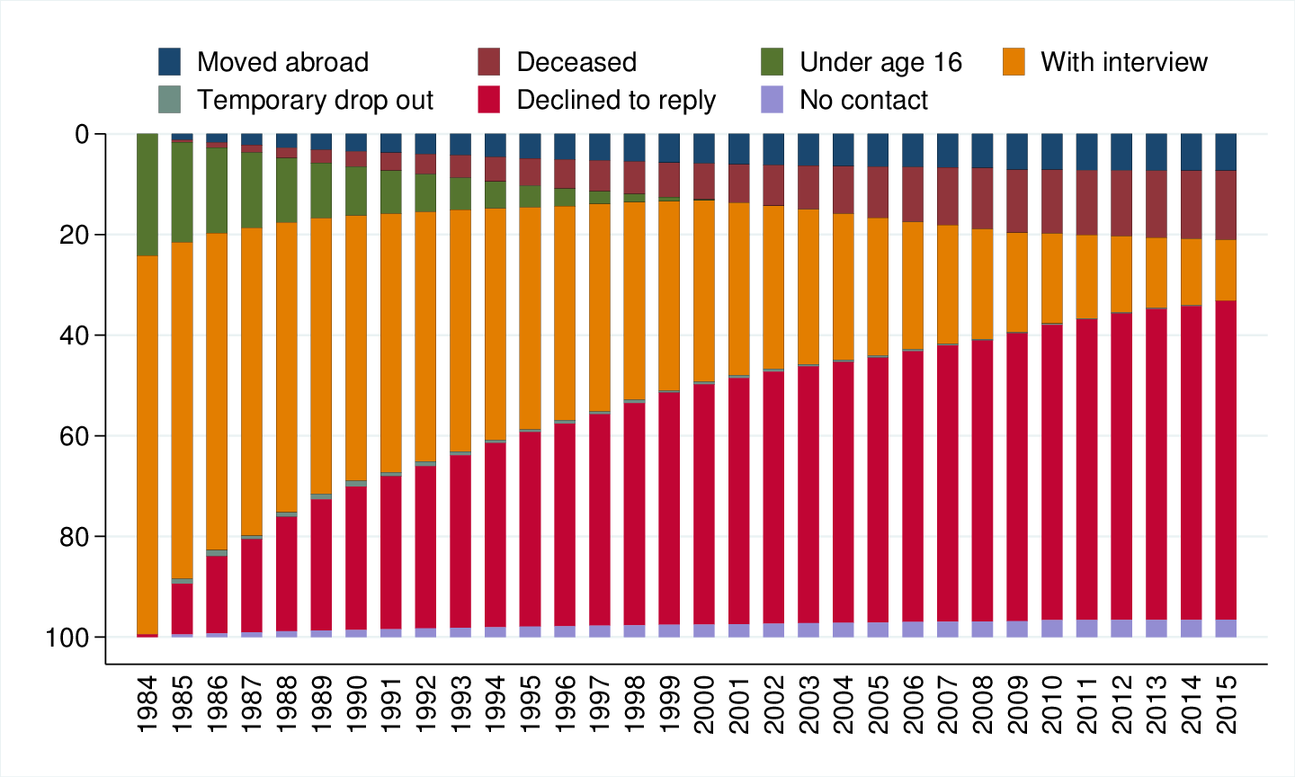
This cross-sectional view is insufficient when examining the longitudinal development of the sample, which is influenced by different demographic and field-work related factors. As already shown in Table 3, demographic reasons for entering the panel are birth and residential mobility. Analogously, the demographic reasons for a panel exit are death and moving abroad. Fieldwork related reasons are different, in that they relate to the interaction between the interviewer and the responding household. Respondents are either not reached for an interview (non-contact) or they decline to participate for the current year. Figure 4 illustrates the longitudinal development of first-wave respondents in 1984, as well as their children, of samples A and B.
Figure 4: Longitudinal Development of the 1984 Population